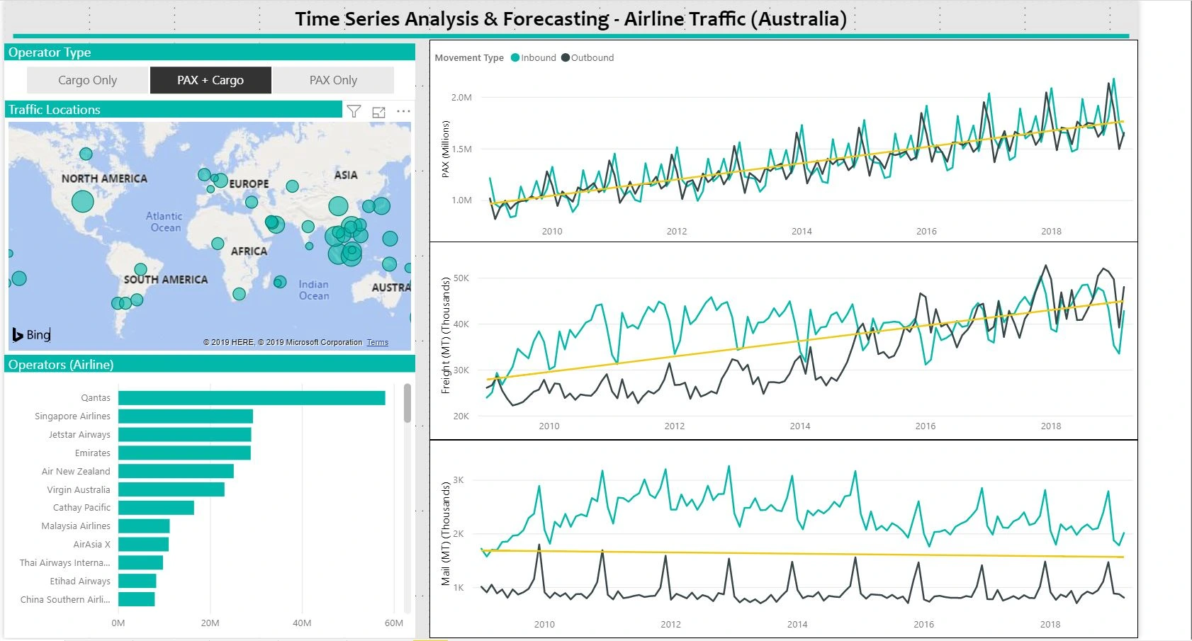

Overview of Long-Term Trends
Three different measures show vastly different trends and seasonality patterns.
- PAX: Predictable Seasonal & Positive Growth
- Freight: Quasi Seasonal & Positive Growth
- Mail: Predictable Seasonal & Flat Growth
Two main components within time series analysis are ‘Long Term’ trends and ‘Seasonal Patterns’.
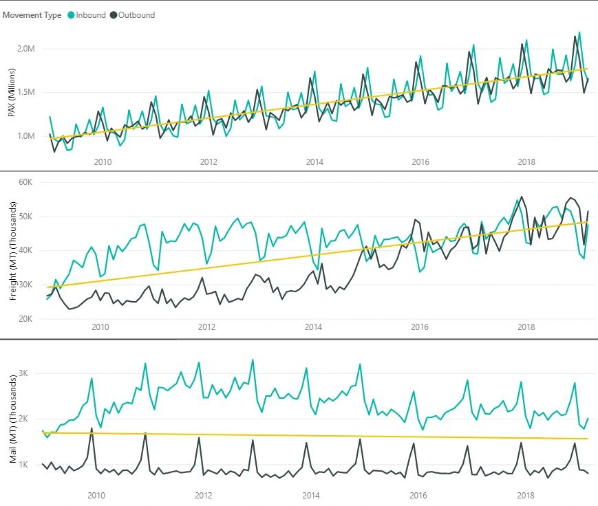
Long Term Trends for PAX show a gradual increase in traffic and seasonal patterns are consistent across different holidays across the year. An interesting observation between movements shows a lag in outbound traffic preceding inbound traffic.
Freight also grows gradually over the long term with seasonal fluctuations. Compared to recent years, the flow of freight into the country overshadowed outbound shipments. This difference has narrowed and consolidated in recent years.
Mail traffic is flat with steady slightly similar to PAX patterns. The quantum of mail entering the country is constantly above the mail volume moving out.
The additive model can be used across all measures as the seasonality pattern does show fluctuations that are within boundaries.

Observations made earlier on aggregated data only partially conform for individual locations and/or operators.
Apart from seasonality, there are several additional factors that influence traffic patterns for a specific location and/or operator.
In the current context, PAX and Freight movements are similar to previous observations with aggregated data, but Mail traffic is drastically different.
An in-depth look at patterns
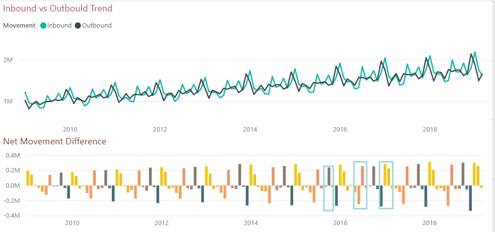
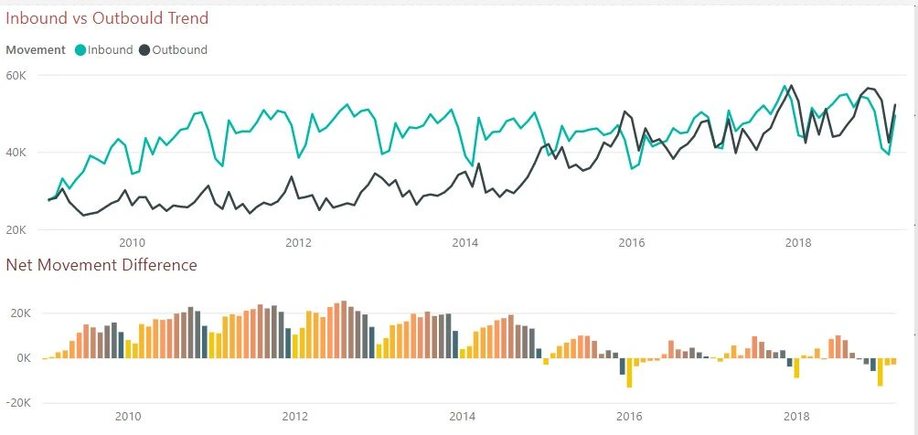
Passenger trend has a predictable pattern where there are certain periods of the year that indicate the direction of traffic.
The outbound trend has a distinct lag against Inbound passengers indicating the seasonality shift of passenger traffic and a key influencer metric.
Net Passenger movements have distinct patterns between Inbound and Outbound across all years. Highlighted in the chart are December-January-February & June-July
Apart from the cycles above, a solitary spike in Inbound was observed for October consistently across the years.
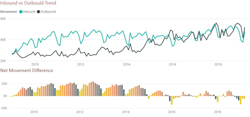
Cargo (Freight and Mail) also exhibits seasonality patterns similar to passengers. With Freight contributing 96% and Mail 4% towards Cargo, the cumulative value dominates the trend of Freight traffic. Net Mail has always been positive indicating more incoming than outgoing mail, whereas Net Freight has an equalizer pattern for recent years compared to prior years.
Mail:

Cargo:
Freight:
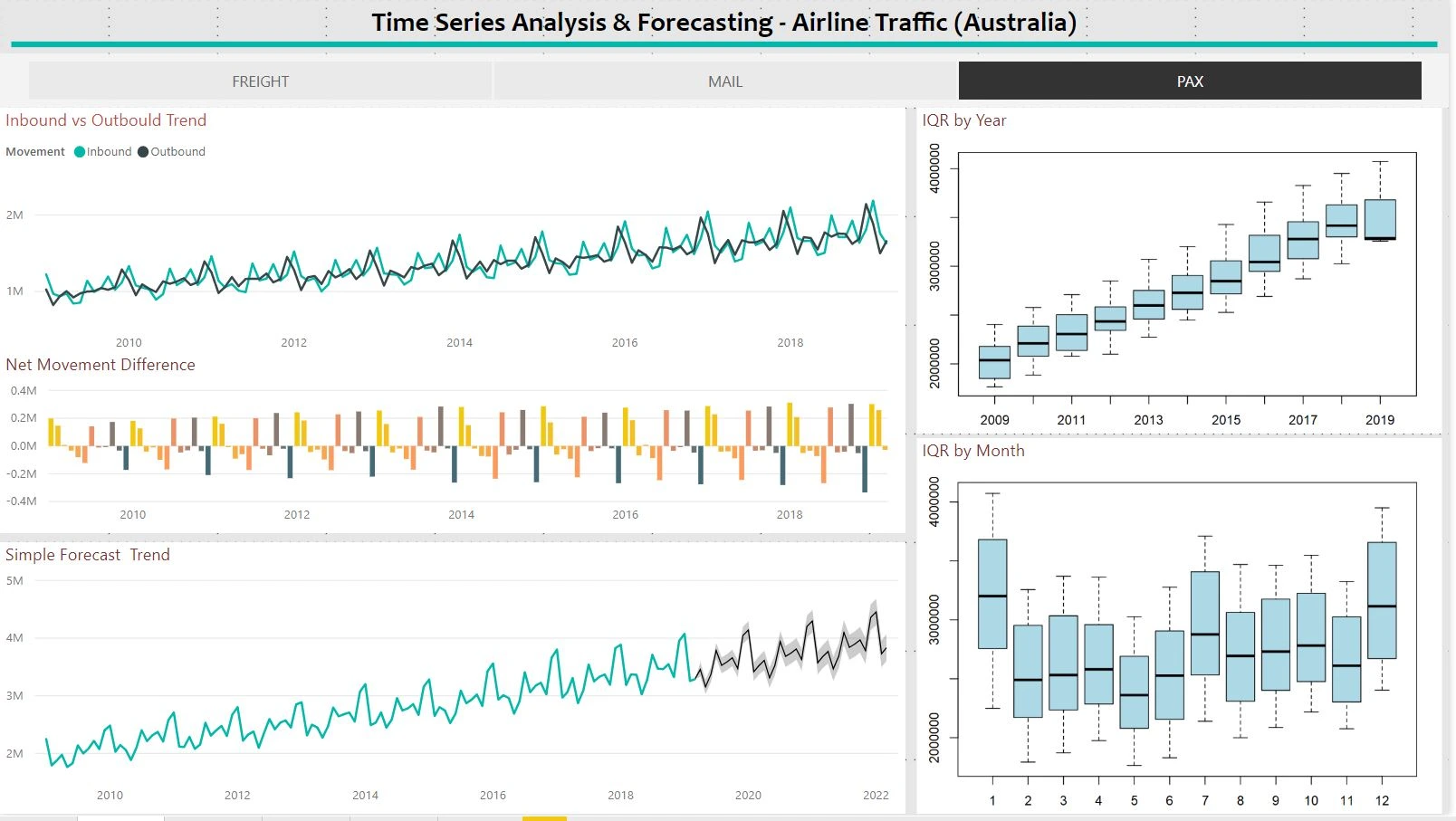
Distribution of values
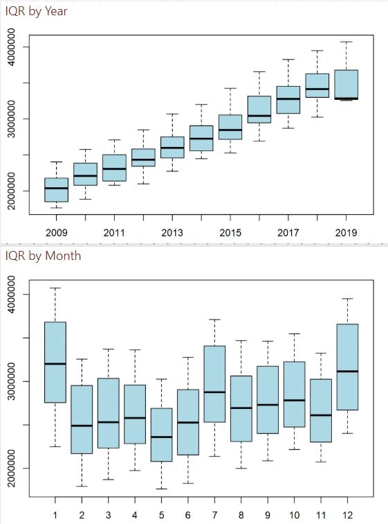
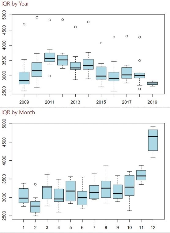
The distribution of values for various measures plotted for Year and Month shows the seasonality of measures, outliers, and spread of values for various data points. Data for 2019 can be ignored due to partial year data.
- PAX distribution across years is constant with a steady increase in Mean value without any outliers. In monthly distribution, the months of January, December, and July are different from other months, which was identified in the earlier Net PAX trend graph.
- Freight distribution is similar to the PAX trend from the yearly perspective with even distribution of values and a steady increase in Mean value. Monthly values do not show significant deviations, which could change in the future due to the drastic change in Inbound and Outbound freight characteristics in recent years.
- Mail data has outliers that coincide with steep spikes seen in the previous graphs. In yearly and monthly perspectives, the pattern is erratic, which might end up in large error coefficients during prediction.
PAX:
Mail:
Freight:

Methods of forecasting
Previous analysis of data patterns implies that the data set is of additive time series nature. Common methods of forecasting include Mean (AVG), Moving Average (MA), Weighted Average (WA), and Exponential Smoothing (ES) mechanisms. In an ideal scenario, the prediction model to be adopted should be able to predict for multiple periods into the future. These simple methods such as MA, WA, and ES can predict only one future data point with accuracy.
In a time series data model with the seasonal component, two popular prediction methods are Holt-Winters and ARIMA (Auto Regressive Integrated Moving Average) models. Time series data is first segregated into Overall Trend & Seasonal Patterns and prediction logic is applied to both components individually.
Standard Power BI forecasting functionality uses the Exponential Smoothing method for prediction.
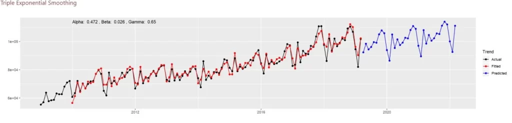
Holt-Winters – Triple Exponential Smoothing
In this case, R standard libraries are used to plot the Holt-Winters method for predicting the values for the next 3 years (n = 36). The best fit of the various coefficients (alpha, beta & gamma) is determined by minimizing the overall SSE of the model. The section below shows the Holt-Winters model for two measures as follows:
- Actual (Black): Actual traffic values from the dataset.
- Fitted (Green): Based on coefficients, the fitted model shows the degree of accuracy.
- Predicted (Blue): Based on coefficients, the predicted values for future periods.
PAX:

CARGO:
ARIMA (Auto Regressive Integrated Moving Average)
ARIMA forecasting method splits the time series into three components (a) Auto-Regressive (b) Integration and (c) Moving Average. R has a handy function called auto.arima to be used alongside the ARIMA algorithm. This function iterates through different parameters and provides the best-fit coefficients with minimal residuals.
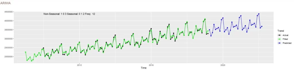

ARIMA prediction outcome is similar to the output of the Holt-Winters model. The exact values for both models might slightly vary. In order to finalize the best model with the highest accuracy, one can split the data into training data up to 2017 from historical data tests against 2018 & 2019 in order to fine-tune various parameters.
Both models fit the values slightly differently. In the Holt-Winters model, the fitting lag is 1 year i.e., 12 months as our time series data grain is monthly. In the case of the ARIMA model, the fitting process includes all data points without skipping any data point.
Other resource:
Time Series Analysis of Passengers – Air Traffic Analytics – Case study