Linear regression is a statistical approach used to model the relationship between a dependent variable and one or more independent variables by fitting a linear equation to observed data.
Linear Regression in Time Series
“Time” dimension in an analytical context is always forward looking and equally incremented. In this context, linear regression helps us understand how any independent variable is influenced against the dependent variable i.e. time period.
Assumptions in Linear Regression
Linearity : The independent and dependent variables are related in a linear fashion. This suggests that changes in the dependent variable (s) are linearly followed by changes in the independent variable(s).
Independence : The observations in the dataset are unrelated to one another. This signifies that the value of the dependent variable for one observation is independent of the value of the dependent variable for another.
Normality: The errors in the model are normally distributed and the variance of error is constant
No multicollinearity: There is no high correlation between the independent variables. This indicates that there is little or no correlation between the independent variables.
Example
Equation of Linear Regression
Y=a0+a1*X
X is the independent variable and it is plotted along the x-axis.
Y is the dependent variable and it is plotted along the y-axis
Values of a0 and a1 are calculated using the below formulae
a1=((xy)`-x`y`) / (x2)`-x`2
a2= y` – a1 * x`
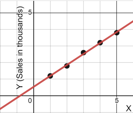
Let X stand for the week and Y stand for sales.
X(Week)
Y(Sales in thousands)
1
1.2
2
1.8
3
2.6
4
3.2
5
3.8
X
Y
x²
X*Y
1
1.2
1
1.2
2
1.8
4
3.6
3
2.6
9
7.8
4
3.2
16
112.8
5
3.8
25
19
SUM
15
12.6
55
44.4
AVERAGE
X`=3
Y`=2.52
(X2)`=11
(XY)`=8.88
a1=0.66 , a0=0.54
Regression equation : Y = a0 +a1*X
Y = 0.54 + 0.66X
Dataset Information
The sample dataset from the Industry schema is as follows, with a focus on the “salesorderheader” relation.
Field
Type
Candidate Variable
OrderID
Character
CustomerID
Integer
ShipDate
Timestamp
✔
SalespersonemployeeID
Integer
ShipMethodID
Integer
TerritoryID
Integer
SubTotal
Numeric
✔
Number of records : 1561
Candidate keys
Number of unique values
Max Value
Min Value
Subtotal
623
129,261.254
2.29
ShipDate
675
2014-05-01
2011-06-01
Workflow
Reading & Manipulation of data
The data is read via DB connector node and fed into KNIME via DB reader after choosing appropriate relation and extracting the necessary primary candidate key.
SubTotal values are grouped by applying an aggregate function sum, and this grouping is based on week, month and year.
Convert the time variable to incrementing integer to overcome tool restriction
Prediction
Execute the “Linear Regression Learner” node on the data present in the “SubTotal” column for the weekly and monthly data.
Add the number of prediction nodes for the prediction step. The granularity of source data is maintained here.
Execute the “Regression Predictor” node on the weekly and monthly data.
Visualization
Monthly data
Monthly data : green line → best fit line
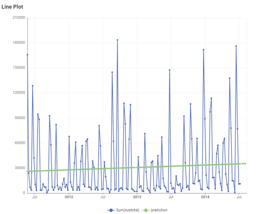
Weekly data
Green line → best fit line
Forecast Accuracy
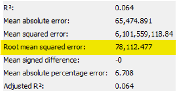
Monthly data
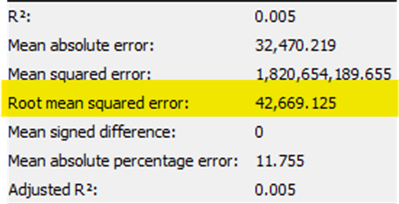
Weekly data
Conclusion
Linear regression is used to establish and quantify the relationship between a dependent variable and one or more independent variables.
Predicting and understanding the behavior of the dependent variable based on the values of the independent variables.
A Lower RMSE Value indicates best fit line
There is a higher RMSE value in monthly data suggests that the line is not best fit
Based on the two observations observations above it is imperative that wide variations in data points leads to poor accuracy
Eliminating outliers can improve accuracy but it should not impact the stability of data