Introduction
In the realm of time series data analysis, the weighted moving average emerges as the next progression to simple moving average, capable of unraveling patterns with additional parameters. Unlike its traditional counterpart, this technique assigns varying degrees of importance to individual data points, granting us the ability to emphasize the significance of specific periods in the forecast.
What is Weighted Moving Average (WMA)?
Weighted moving average is a statistical calculation method that assigns different weights to individual data points in a time series. These weights reflect the relative importance of each data point in the average calculation, allowing for a more nuanced analysis that emphasizes certain periods or events over others within a time window. This technique is particularly valuable in capturing trends and patterns that might be obscured by a traditional, simple moving average i.e. equal-weighted moving average.
Formula
WMA(T) = [x(T-1)*w1+x(T-2)*w2+…..+x(T-n)*wn]
WMA(T) = Weighted moving average of data point at time T
- x(T) = data point at time T
- w1 ,w2,w3 are corresponding weights
- w1+w2+w3…wn=1
- n is the window length
Example
DAY | SALES | WMA (n=3) |
|---|---|---|
| 1 | 50 | NA |
| 2 | 52 | NA |
| 3 | 55 | NA |
| 4 | 53 | 53.9 |
| 5 | 54 | 53.3 |
| 6 | 56 | 53.3 |
| 7 | 58 | 53.3 |
| 8 | 60 | 57.2 |
| 9 | 62 | 57.2 |
| 10 | 65 | 61.2 |
| 11 | N/A | 63.9 *predicted value |
| 12 | N/A | 19.2 *Predicted value *deteriorated value |
Key Considerations:
- In this scenario, the assigned weights are 0.1,0. 2, and 0.7, while the window length is set to 3. In this case, the most recent data in the time window has more weightage compared to slightly older periods
- Forecasted data is limited to a single period, regardless of window size.
- Precision of the forecast is tied to the number of periods.
- Deterioration in data quality is evident when making predictions beyond one period.
- Data degeneration is attributed to the existence of null values in the actual column
Dataset Information
The sample dataset from the Industry schema is as follows, with a focus on the “salesorderheader” relation.
Field | Type | Candidate Variable |
|---|---|---|
| OrderID | Character | |
| CustomerID | Integer | |
| ShipDate | Timestamp | ✔ |
| SalespersonemployeeID | Integer | |
| ShipMethodID | Integer | |
| TerritoryID | Integer | |
| SubTotal | Numeric | ✔ |
Number of records : 1561
Candidate keys | Number of unique values | Max Value | Min Value |
|---|---|---|---|
| Subtotal | 623 | 129,261.254 | 2.29 |
| ShipDate | 675 | 2014-05-01 | 2011-06-01 |
Snapshot of the data

Workflow Details

In the KNIME platform, access the dataset and extract the pertinent columns for analysis. Data is grouped and cleaned so that the “SubTotal” column can be used to calculate Weighted Moving Average. After computing the weighted moving averages including forecasting, a visual representation of the baseline and predicted data highlights the outcome.
Reading & Manipulating Data
- The data is read via DB connector node and fed into KNIME via DB reader after choosing the appropriate relation and extracting the necessary primary candidate key.
- SubTotal values are grouped by applying an aggregate function sum, and this grouping is based on month and year.
Forecasting
- Execute the Weighted Moving Average methodology in the data present in the “SubTotal” column.
- Initialize variables that stores assigned the weights
- The allocation of weights is designed to prioritize recent data points, with emphasis intensifying progressively. The assigned weights follow a sequence of 1.2 and 3 with 0.1, 0.2 & 0.7 weights wherein the time window size is 3.
- Calculate the Weighted Moving Average by traversing time period and multiplying with corresponding weights as predicted values.
Imbalance in assigning weights in systemic patterns may result in incorrect prediction. For e.g., if data has a periodic increase in weekends vs. weekdays, the weightage of such data points in a moving average must be adjusted accordingly.
Visualization
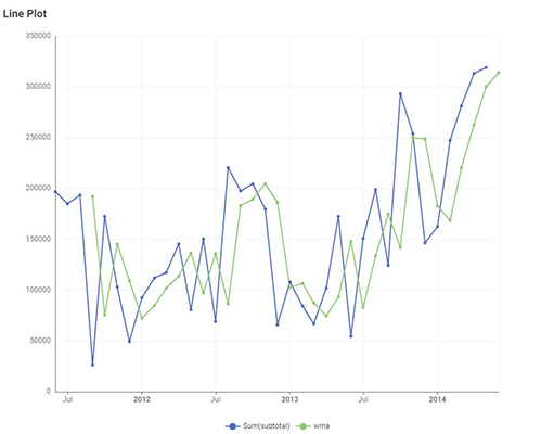
Green line : predicted value of the Subtotal
Blue line : actual data points of SubTotal
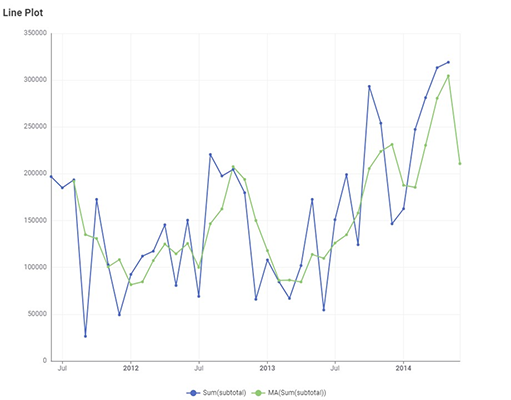
Green line : predicted value of the Subtotal
Blue line : actual data points of SubTotal
Summary
- Explored dynamic nature of weighted moving averages as a versatile tool for time-series data analysis.
- Compared with Simple Moving Averages by incorporating varying weights. A stark difference noticed in the outcome of the forecast between SMA and WMA
- Emphasized the strategic weight assignment based on data patterns, thus enhancing trend accuracy.
- Stressed context-awareness for interpreting predictions and ease at which they can be applied in planning and forecasting use cases across industry sectors