What is Planning?
Activities are done by all organizations across functional domains and industry verticals. Based on historical data, current performance, market trajectory, and a host of other factors teams set targets for subsequent years. Values such as budget, forecast, and stretch are arrived at and published. Subsequently, the budget and forecast are tracked against actuals on a monthly basis and performance is tracked. If the need arises, values are re-adjusted after approvals are received.SAP Analytics Cloud – Planning
 SAC Planning models facilitate generating collaborative Budgets, Forecasts and integrate with realized actuals from enterprise systems on a near real-time basis. Planning and forecasting accuracy can be improved with advanced features such as Variance management, Value Driver Tree, Predictive Modeling, and integration with R.
SAP Analytics Cloud uses two different kinds of models that follow a simple star schema approach
SAC Planning models facilitate generating collaborative Budgets, Forecasts and integrate with realized actuals from enterprise systems on a near real-time basis. Planning and forecasting accuracy can be improved with advanced features such as Variance management, Value Driver Tree, Predictive Modeling, and integration with R.
SAP Analytics Cloud uses two different kinds of models that follow a simple star schema approach
- Analytical Model – Reporting and Data Visualization
- Planning Model – Reporting and Planning
Granularity
Any entity or dimension is said to be of high granularity when the total number of unique values is large. E.g., Dataset with ‘Date’ values is of high grain when compared to a dataset with ‘Year’ values alone.
Cardinality
It is related to cardinality and is defined as the number of unique values for an entity or dimension. This defines rows in one table that match those with structured linkages, such as one-to-one, one-to-many, and many-to-many, between other tables or entities.
The number of entities or dimensions, their cardinality, and the granularity of each entity drive the complexity of the data modelAggregation
Aggregation methods define how measures behave during calculation at run-time. It depends on the selected entities and cardinality wherein one cumulated row of output for each granular combination is computed for aggregate functions such as Average, Sum, and Count. SAC supports restricted and exception aggregation that is unique in runtime behavior. These aggregation types require entitie(s) associated with measures and are triggered only when associated entitie(s) are included in the calculation context.Hierarchy
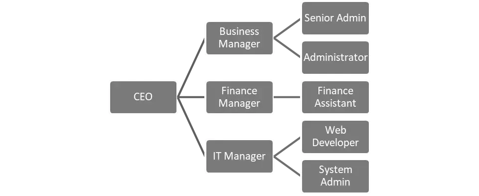
Hierarchy is a specialized data structure that shows tree-like structures and relationships between roots, branches, and leaves. SAP Analytics Cloud supports two types i.e., Level based and parent-child hierarchy. The hierarchy type is decided based on requirements and data availability, but the behaviour is identical from a reporting and planning perspective.Data Loading Behavior
We created a model using a simple use case related to Sales Planning with the following Dimensions and Measures- Date – Month Granularity with YQM default hierarchy
- Product – With additional properties (attributes) such as Category, Brand, SubCategory, MSRP, etc
- Location – With additional properties such as LatLong, Region, Country, etc
- Revenue and Quantity as standard measures with SUM as the default aggregation method
Summary of data load behavior
| No | Type | Use Case | Observation |
| 1 | Data Load | Public dimension data load Process key and description in two data load sequences. Each data load has distinct set of records without any overlap | All values inserted into dimension. Each distinct dataset is treated as an UNION operation and appended into the dimension |
| 2 | Data Load | Public dimension data load Process key and description in two data load sequences. Second data load has distinct set of records without any overlap and few records from first data load | All distinct values are inserted into dimension. Any repetitive value is updated accordingly UPSERT is the default behavior based on the key column |
| 3 | Data Load | Public dimension with 2 properties. Process key, description and one property in first load. Second data load has key, description and second property with overlap to first data load | All unique values are inserted and repetitive values are updated. Default value i.e unmapped data is blank. UPSERT action ensures that all properties are updated including description |
| 4 | Data Load | Model with 2 Public Dimensions and 2 Measures. Load dataset with existing values in dimension master data and new value | Only matching members are loaded into the model. Invalid members are ignored and must be updated in the public dimension directly first before loading into model. |
| 5 | Data Load | Model with 2 Public Dimensions and 2 Measures. Default dimension Date is a Local i.e. Not Public dimension at all times Load first dataset for MeasureA. Subsequently process MeasureB in the second data load with the same cardinality. | Initial run processes data and populates values of the first measure and the second measure is filled with null values. Second measure was updated with values after the second load. Model loading follows the UPSERT principle. Important factor here is the cardinality of model, unlike dimensions where key played major role |
| 6 | Data Load | Model with 2 Public Dimensions and 2 measures. Create two public versions public.Actual & public.Budget. Prepare and load data for all dimensions and measures for public.Actual version in first run and load the exact same dataset without any changes except for version public.Budget in a second run. | Both loads loaded the exact same data without any changes to different versions. Model type i.e. Analytics vs Planning controls version dimension. Analytical model will behave similar to previous use case (#4) Note: Version is an independent dimension critical for planning and a mandatory entity for SAC planning scenarios. |
Authors
- Vignesh M
- Karpagam K.